
This is an old revision of the document!
Layer Model QC
This tutorial shows selected statistics for a voxel model.
useful for layered models based on boreholes and geopphysical data e.g. 1d models. Used for quality control of correlation between data and model interpretation.
Requirements:
- Layered model
- Borehole data
- 1D geophysical data e.g. resistivity
Step 1. Borehole content
1. See Setting Up Data for Modelling
- Adding point layers
- Interpolation of XYZ points (2D grid)
- Creation of solid layers + definition of bottom/top layers

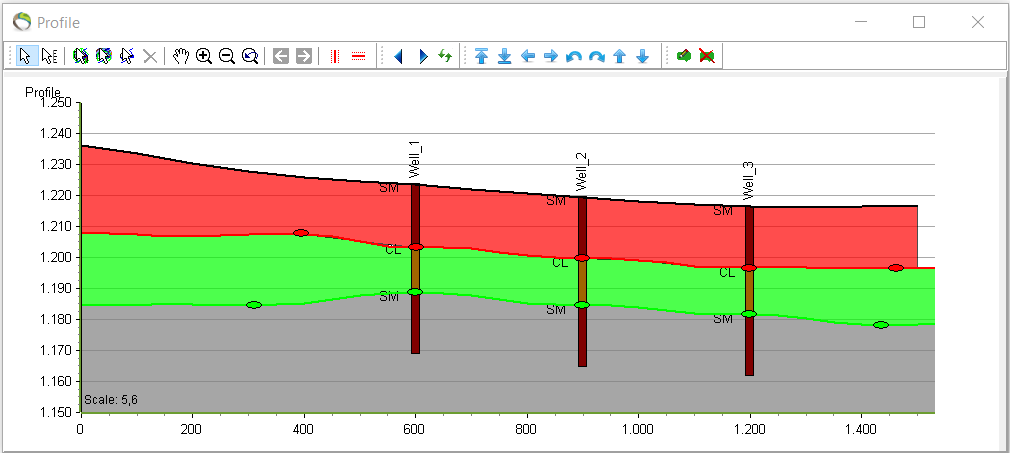
- After adding and interpolating XYZ points to XYZ layers (2D grid) and creating solid layers the profile looks like the picture below.
2. See Edit XYZ Points - In Profile Window
- Edit point layers
- Interpolation of layer points (edit 2D grid)
- Moving layer points
- This GeoScene3D tool is used for checking whether a lithology from the borehole data is corresponding to the interpolated XYZ layers. Here clay is chosen.
3. QC and Statistics menu –> “Layer Model QC” –> next –> “Calculation Mode: Wells” –> clay.
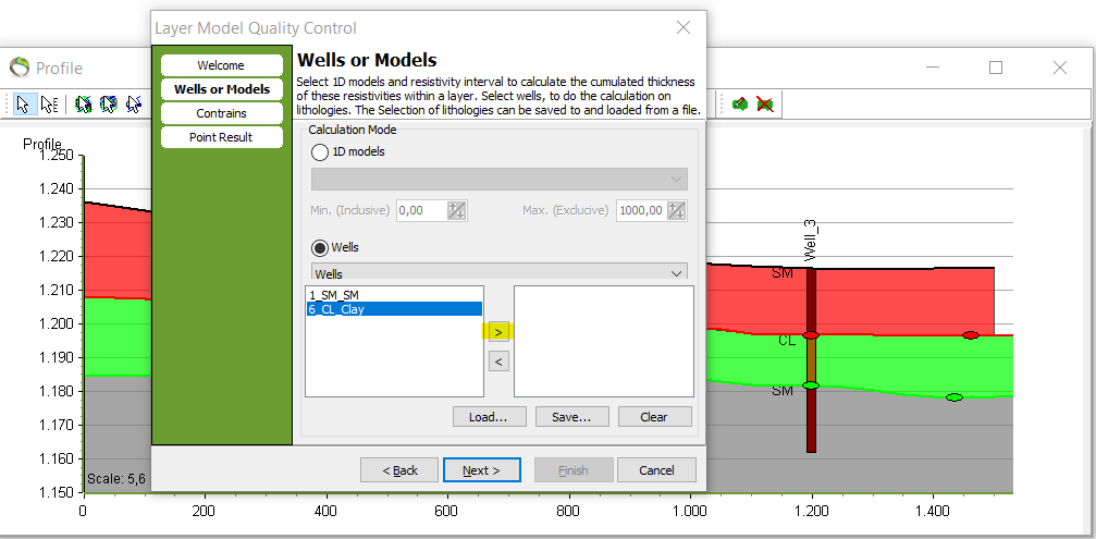
4. Define the constraints for the bottom and top of the surrounding layers –> next –> finish.

5. Activate the top plot in the profile.
- The top plot y-axis marks the clay thickness (total overlap) while the color of the points demonstrate the clay content percentage in the constrained interval (percent overlap).
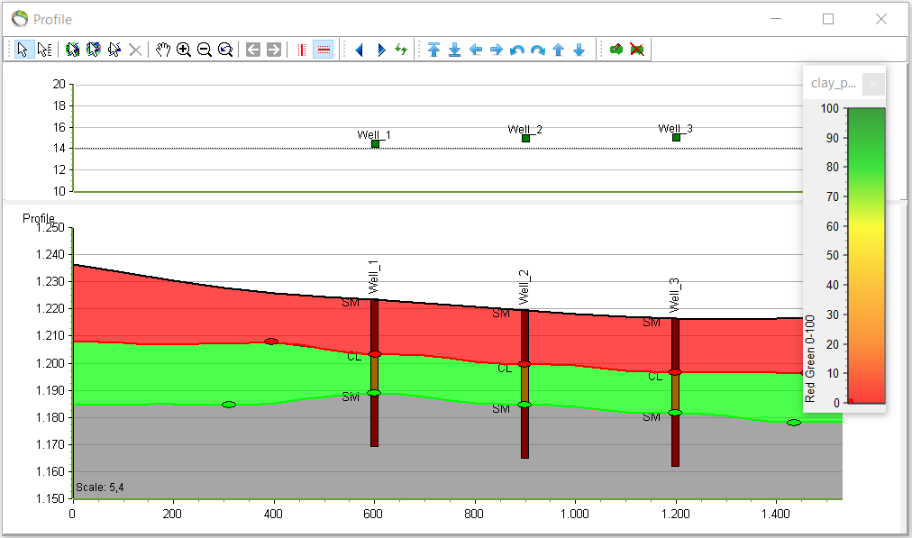
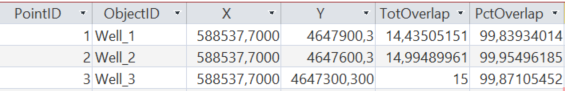
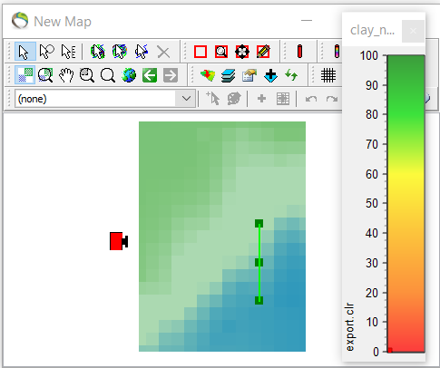
- The point information can also be opened in a file, MS Access Database. Here the clay content is almost the same as 100% (dark green) from the picture above.
- The points can also be applied to the map to get an overview above the prevalence of the points.
- Constraints are not neccesary if information about the entire well is wanted. E.g. if information about sand content is wanted the sand percentage will accordingly be lower if more than one lithology is present in the well.
- In the next pictures there are no constraints. The light green top points correlate to sand whereas the bottom orange points correlate to clay content in the entire well. About 85% sand in all boreholes and a total thickness of 40 meters. Accordingly about 15% clay in all boreholes and a total thickness of 15 meters.
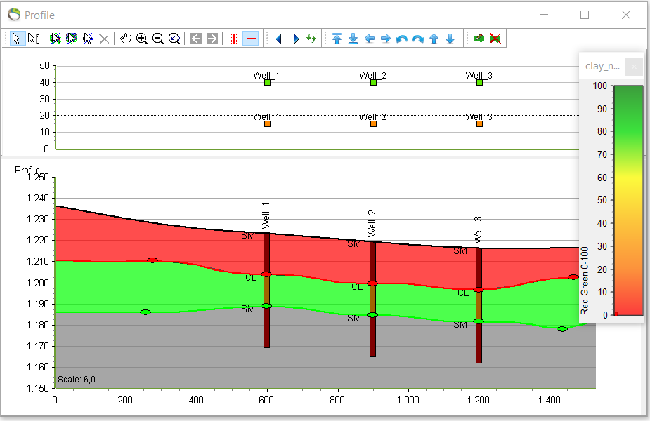
- In the next photo the data is manipulated to show how data behave if the correlation is not correct.
- In well_1 the points is red correlating to 0% of clay in the green solid clay layer.
- In well_2 there is 100% of clay and the layer is 10 meters.
- In well_3 the clay content is about 20% and the layer is maybe 13 meters.

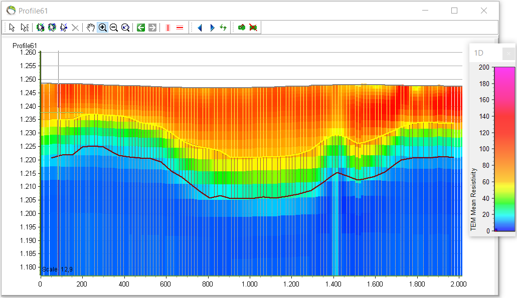
Step 2. 1D modeller
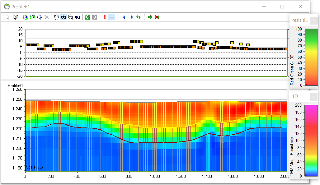
- The layer model QC can also be applied to 1D data e.g. for resisitivity.
1. Repeat step 1.3. and click “Calculation Mode: 1D models” –> define the resisitivity interval –> next.
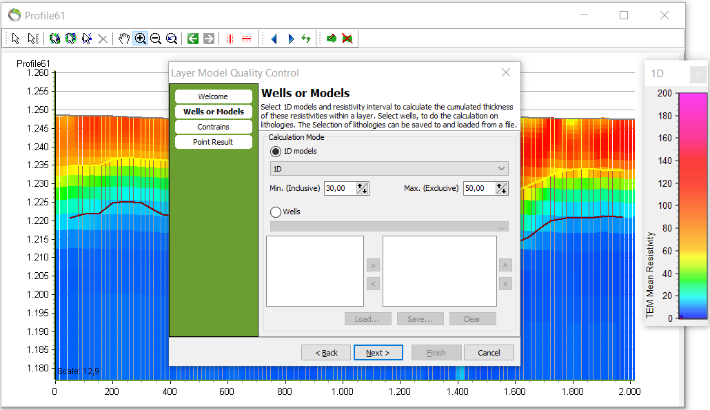
2. Repeat step 1.4. for constraint definition.

3. Repeat step 1.5. and fit the top plot to the data.
Step 3. Result
