
This is an old revision of the document!
3D Grid Histogram
This tutorial shows how to quality check data by making histograms. The histogram can be used as a tool to gain a data overview before model building but the histogram is also useful for checking correct correlation between different datasets. Thus, it is a useful tool for analyzation both before and after model building.
Requirements:
- Voxel model with 3D grid
Step 1. Floating value 3D Grid histogram
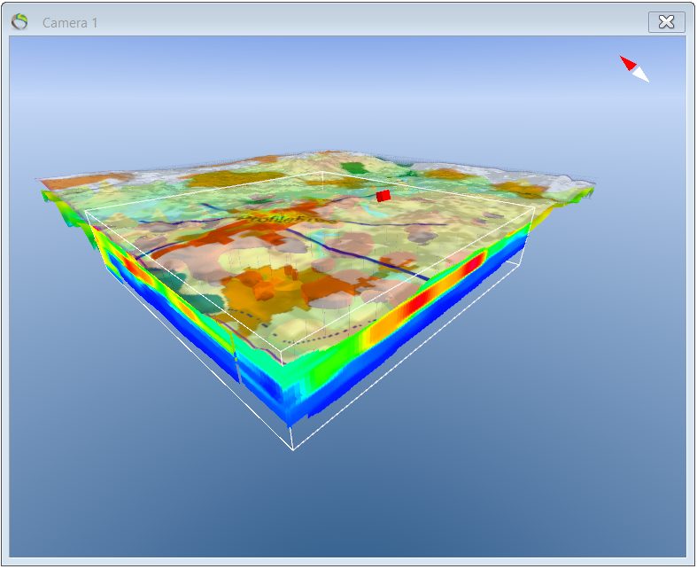
- To make histograms a voxel model is needed.
- The biggest trends of a dataset can be visualized and analyzed in the histogram before a model is made by showing the amount of present voxels for different values in the dataset e.g. for resistivities.
- Also, 1D models can be interpolated into 3D grids with the aim to check if data are corresponding e.g. to resistivities.
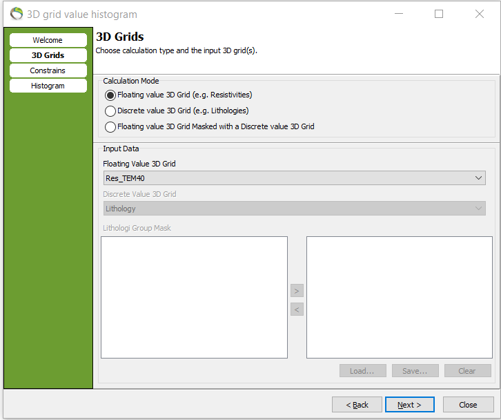
1. “QC and Statistics” menu –> next –> “Calculation Mode” –> Floating value 3D Grid (e.g. Resistivities) –> “Input Data” –> your 3D grid –> next.
2. Choose the surfaces for where the calculation is needed by clicking the upper and lower constraint –> next.

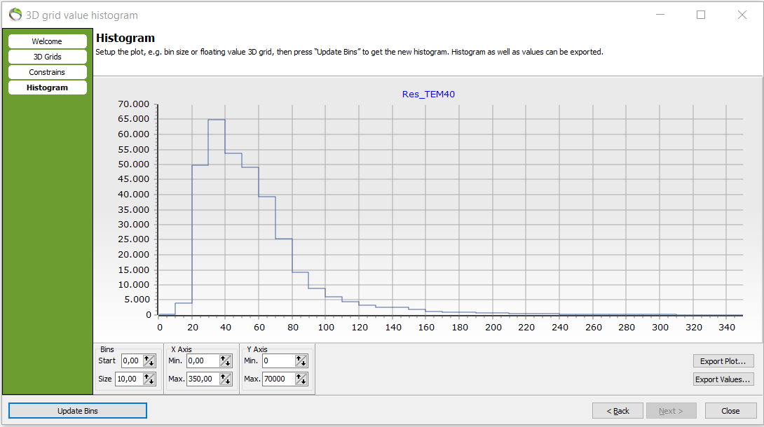
- A histogram has been made that shows voxel counts (y-axis) against resistivity (x-axis).
3. The histogram can be exported as an image “export plot” or as values “export values”.
4. The axis values can also be changed.

- In the following picure the axis values has been fitted to the datapoints.
- Notice how the bin size can be edited. Here, e.g. there are 65.000 voxels in the resistivity interval [30;40].
- The bin size has been changed from 10 to 20. The degree of details has been decreased but the following voxel count has increased in the bigger resistivity interval e.g. 115.000 voxel counts in the resistivity interval [20;40].

Step 2. Discrete value 3D Grid histogram
- Discrete values e.g. chemistry values or lithologies.
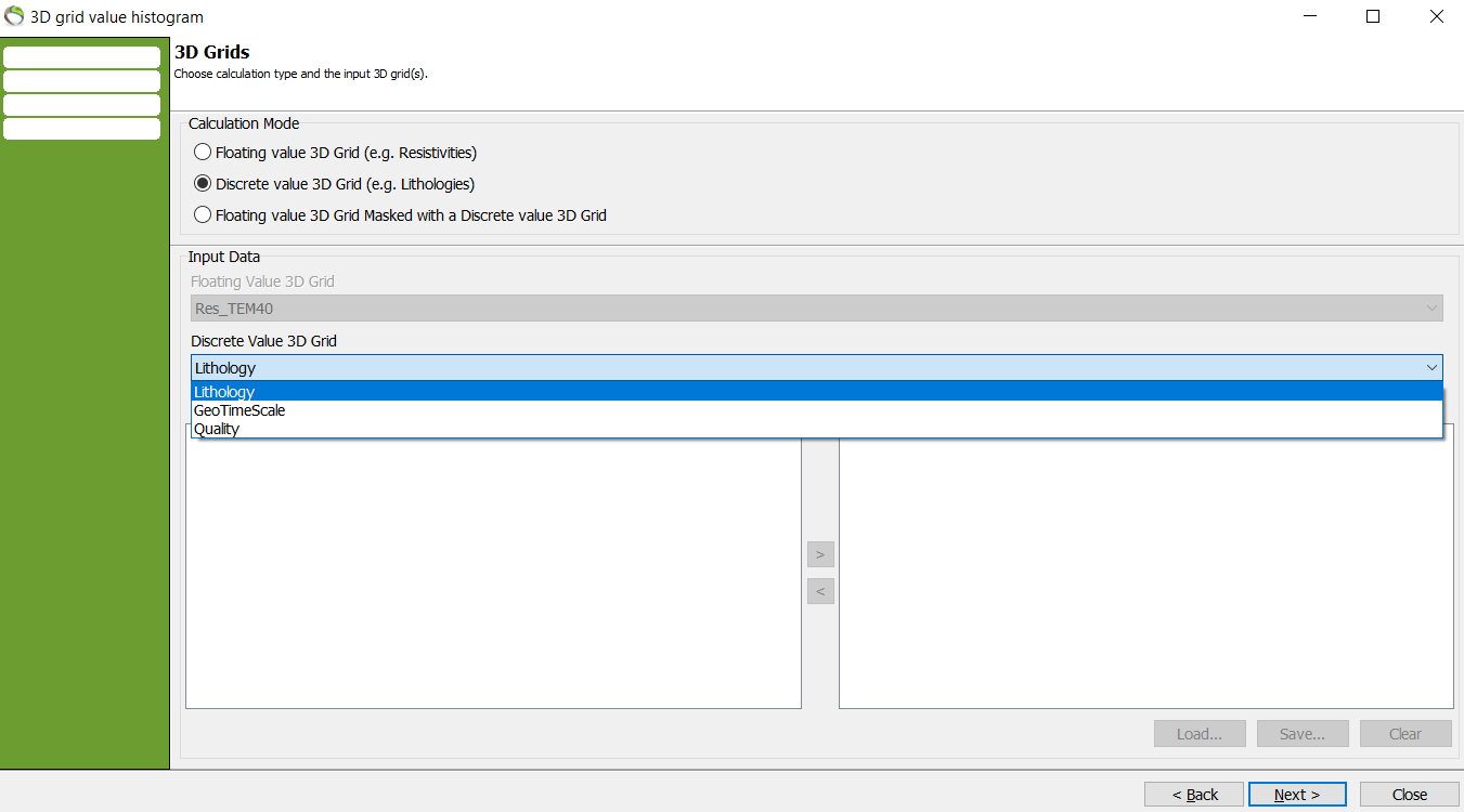
1. Repeat step 1.1. but choose “Discrete value 3D Grid (e.g. Lithologies)”.
2. Pick the discrete value for the histogram in “Discrete Value 3D Grid”. Here lithology is chosen.
3. Repeat step 1.2. for constraints.
- A lithology histogram has been made.

4. To show the lithology legend go to Object Manager –> rightclick lithology –> show legend.

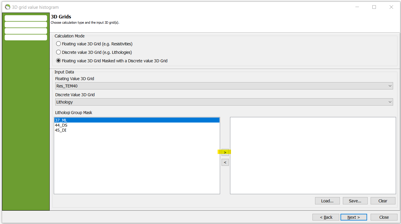
Step 3. Combination of floating and discrete values
- This tool is used to check e.g. if your resistivity data matches the concerned lithology.
- In this histogram setting the resistivities are held together with the lithology at the same voxel position.
you get the resisivities in the 3d grid at the same position as specific matching lithology grid values.
picture: click and next. After define constraints like before.
Histogram. Are the resistivities matching/corresponding the specific lithology chosen?
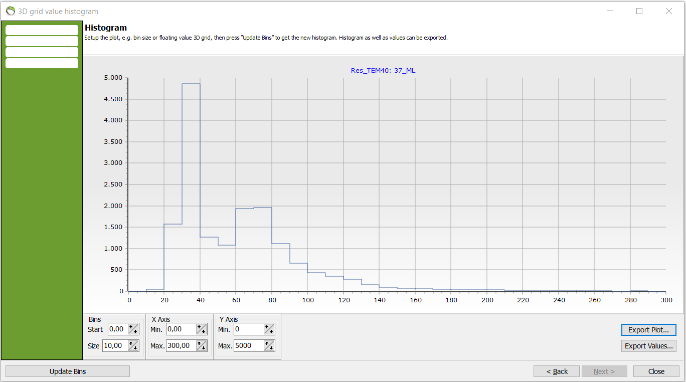
To improve the details of the resistivity in the chosen lithology, the bin size can be reduced e.g. from 10 to 2.

- In previous picture the resistivities are mainly focused around [20;100] ohm*m whereas almost no datapoints are registered after around 150ohm*m.
- The lithology ML (glacial moræneler/leret till = glacial morraine clay) can be expected to withhold low resistivity values and the histogram confirms the expectation. Although, it is distinct that the histogram holds two prominent peaks.
- This peaks need attention. If the voxel counts for the peaks were abnormal and high in the resistivity values for ML something wrong in either the lithology, resistivity values or something that is not in sync.
- in the interpretation of the dataset could be errorneous.