Top Plot

This tutorial contains a video and a written guide how to make and use a top plot from multiple datas. This tutorial operates with pre-made profiles, Jupiter data, XYZ points and layers.

Requirements

• A project with a terrain or grid and a Profil, See Create profile

1. Right clik profile in “Object manager” → “Show Profile Window”.

• To visualize the Top Plot click the icon

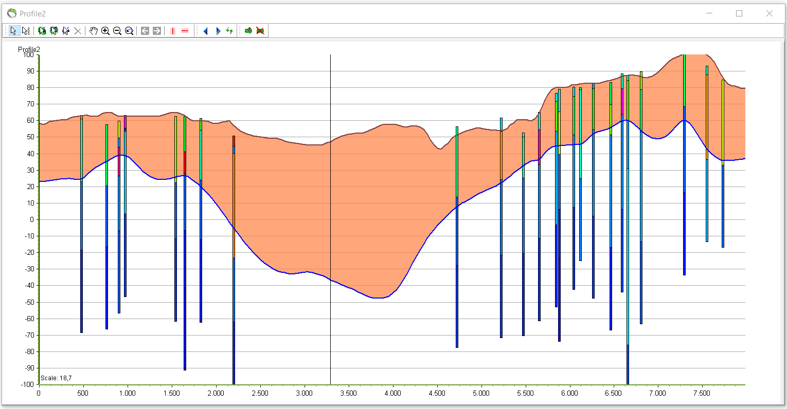
• The Top Plot can be used to isolate cluster information used in GeoScene3D e.g. non-elevated based STD data points for water chemistry together with isopach grid maps.

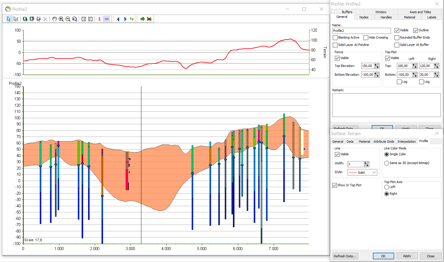
2. Rightclick the terrain in Object Manager → Object Properties → profile click “Show In Top Plot” correct “Top Plot Axis: right” → OK (refresh the profile).

• The color of the curve can be changed in “Material” to emphasize the edit of this particular curve. This can be advantageous if many curves look similar.

3. To edit the terrain elevation in “Profile2” go to Object Manager and right click “Profile2” → Oobject Properties → General → in the Top Plot menu the terrain elevation must be edited on the right side because of the settings made in the terrain properties.

• Note the small blue boxes fixed to the boreholes on previous picture - this boxes can be moved and isolated to the Top Plot.

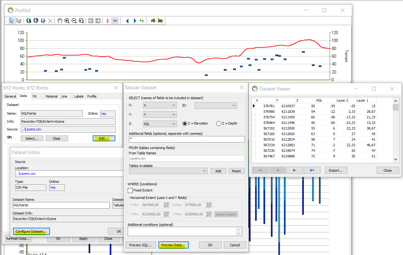
1. Repeat step 2.2. just rightclick the XYZ points in Object Manager and check if the point values are listed on the left side axis.

• To gain knowledge about the value of the data points you need to preview the data.

2. Rightclick XYZ points in Object Manager → Object Properties → Data → Eedit… → Configure Dataset… → Preview Data….

• In the preview for this data, points were observed in the interval between -24 to 116.

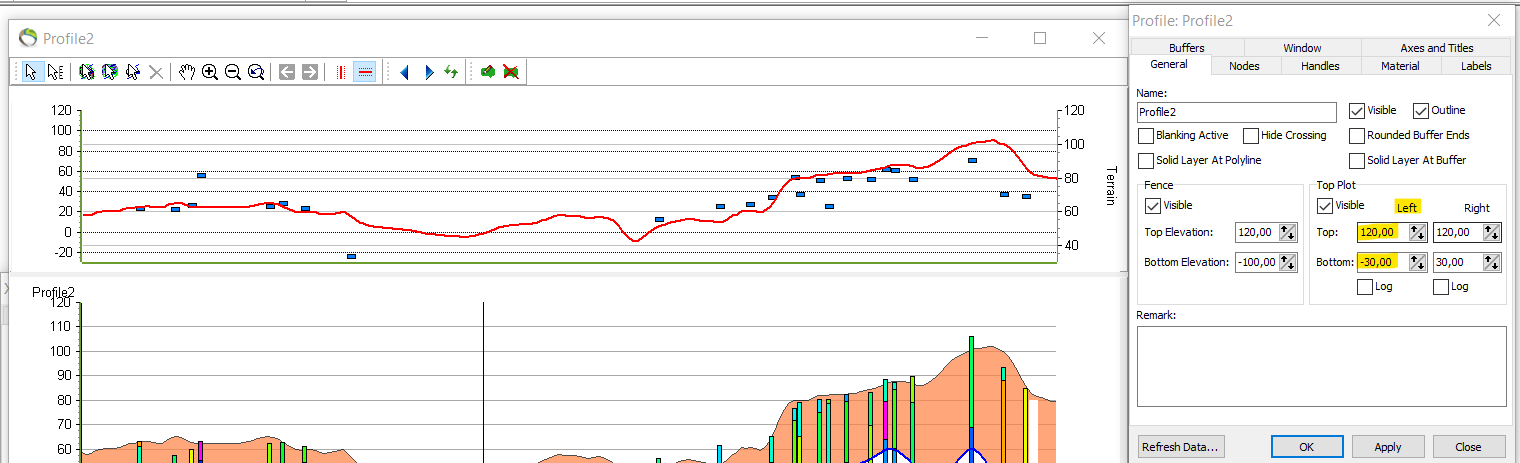
3. Repeat step 2.3. just for the left side axis and check if the axis values need to be corrected according to the values of the XYZ data points.

• The underlying picture demonstrate the edited values on the left axis correlated to the XYZ data points held together with the red terrain curve on the right side axis.

• Lastly, the terrain curve can be clicked back to the profile observed as the red line and a green isopach grid curve (.grd) can be activated to the Top Plot that demonstrates the thickness of the orange layer in the profile. The isopach curve have replaced the terrain curve hence the layer thicknesses can be read on the right side axis.