3D Grid Thickness QC

This tutorial shows how to use voxel models to identify the extent and distribution of specific values (floating values) or specific categories (discrete values) e.g. lithology types. In the voxel model the specific area of interest is evaluated and analyzed within a defined interval where this tool calculates the cumulative thickness of all voxels in all positions with the purpose to visualize the locations of expected values or categories on the map.

Requirements:

• Voxel model

• Voxel model with resistivities.
• Between two surfaces all voxels can be analyzed according to specific resistivity values. To check if expectations matches the reality of the data or if something is wrong with the layer model.

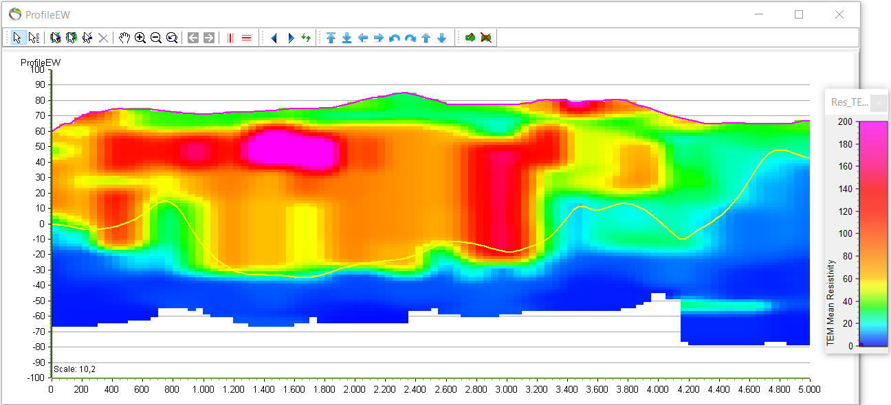
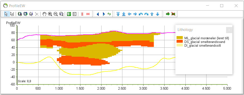
• Open a profile and the according legend and register the range of resistivities.
• Between the terrain (pink) and kriging (yellow) surface in the picture below almost all resistivity values can be observed where the highest values are from about 60ohm*m and up.

1. “QC and Statistics” menu –> “3D Grid Thickness QC” –> next.

2. “Calculation Mode” –> Floating value 3D Grid (e.g. Resistivities) –> pick your 3D grid file.

3. “Min. Value: 60” and “Max. Value: 1000” –> next.

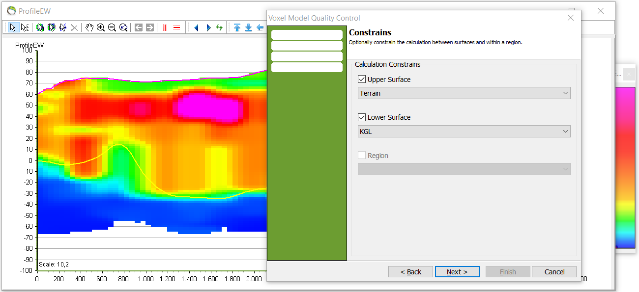
4. You can choose the surfaces for where the calculation is needed by clicking the upper and lower constraint –> next.

• When the constraints are made the tool scans the layer in between for resistivies in the [60;1000] interval.

5. Name the resulting 2D surface –> finish.

• The feature “Add Result to Map” is automatic.
• The new surface can be found in object manager

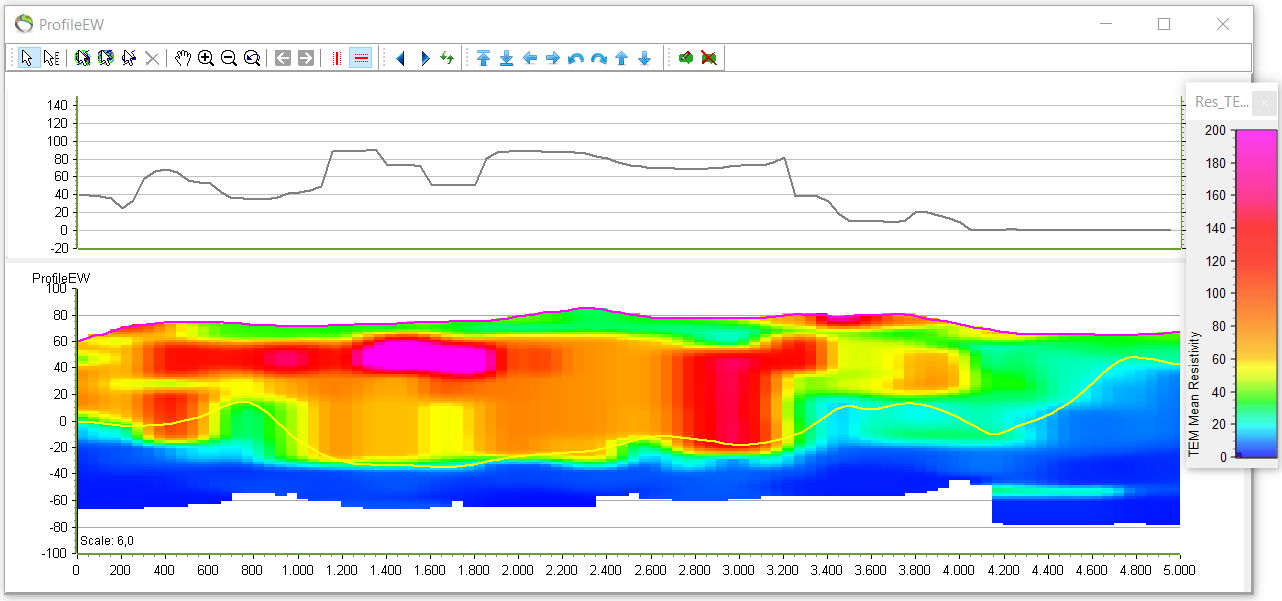
6. Activate the new surface. Also rightclick your profile –> “open profile window” –> “show top chart”.

• The new resistivity chart is visualized in the top plot.
• The y-axis on the top plot show the number of cumulative meters of voxels with the chosen resistivity in the constrained area.

• Analyzing the thickness of the profile in the constrained area for the chosen resistivities
• 60 meters of cumulated voxels having resistivities above 60ohm*m.

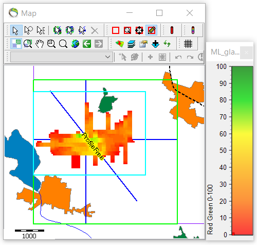
• The picture below show the map before the new resistivity layer was made with interval [60;1000].

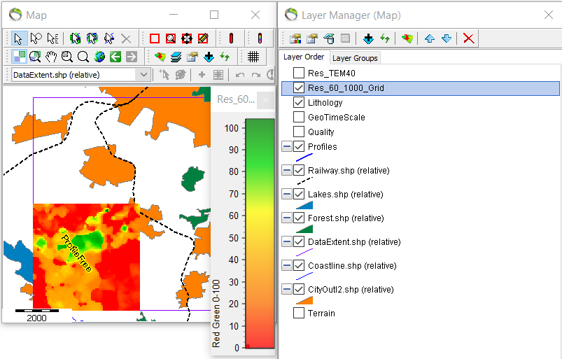
• Next picture visualize the automatic feature from step 5 where the bottom left corner on the map show the different cumulated resistivity values in the interval [60;1000] as an isopach map. In the map it can be observed that the green area contains the biggest concentration of the resistivity interval.
• Note that the colorscale maybe needs to be adjusted to show thicknesses and not resistivity.

• Open profile and activate lithogies and deactivate resisitivites.
• To show the lithology legend go to Object Manager –> rightclick lithology –> show legend.

• Repeat step 1.1.
• Repeat step 1.2. just for discrete values. Pick as many lithologies as wanted for analyzation –> next.

• Repeat step 1.4. for constraints.
• Repeat step 1.5. for naming the new surface.
• Repeat step 1.6. to show the result.

• As before the cumulated voxel thickness is automatically transferred to the map.