This tutorial describes how to use the data transformation features associated with Kriging in GeoScene3D. The tutorial does not explain the mathematical foundation, only the workflow in GeoScene3d.

For more information about basic interpolation and kriging, please look at this presentation.

Why do we need to transform data when kriging?

Many physical phenomena in nature arise from a number of additive variations. The distributions of the individual variations are often unknown; however, the histogram of the summed variable is often observed to be approximately Normal (Gaussian).

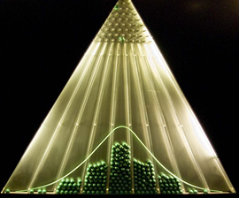
Figure 1. Bean Machine – beans are dropped, and randomly fall into bins. As by magic the Gaussian distribution appears. The more beans, the higher the sampling frequency, the more apparent the bell shaped distribution.

Depending on the amount of data available (the amount of beans in Figure 1), the sampling frequency, you will be able to recognize the characteristic bell shape of the Gaussian distribution.

The Kriging method is based on Gaussian statistics. This means that it is assumed that the underlying data have a Gaussian distribution, a normal distribution, when performing calculating the variogram, performing the kriging, estimating the variance etc..

So, what do you do if your data have another distribution?

Examples could be:

• Chemical measurements. You have a contamination site, with a series of measurements of the concentration of a chemical compound. Such data would typically have a bi-modal distribution, with a large group of measurements (observations) having a very low value, and a separate set of observations having a very high value.
• Terrain surfaces with deep valleys: You have a terrain surface which is relatively smooth, but the area is crossed by deep valley structure, thus leading to a bi-modal data distribution of the elevation observations.

The answer is “data transformation”. You transform the data from “normal” space to a transformed space, where the data have a normal distribution, do the kriging, and then back transform the result.

One type of transformation is the log-transform, another is the Normal Score transform, which is part of the GSLIB library utilized by the program.

See separate documentation for the specific, mathematical details of each transformation.

Startup the interpolation wizard by using the mouse and right-clicking the point object node to be interpolated in the object manager.

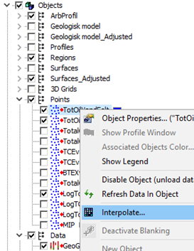
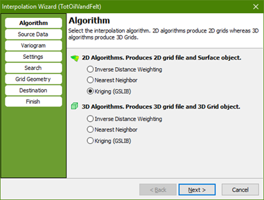
Figure 2. Open the Interpolation Wizard

In the right-click menu, you now select “interpolation”. Step through the wizard as normal, until you reach the “Source Data” page.

Press the “Get Data” button, to select the value to be interpolated. In the example here the value used to color the data points is selected.

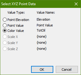
Figure 3 Select the value to be interpolated. Here the color value used for the XYZ points.

On the “Source Data” page, you have tools available for checking the distribution, the statistics, of your data.

Press the “Statistics…” button, to inspect the statistics of the selected value.
Note that if you have a large amount of data, it may take a while to process the statistics of the data.

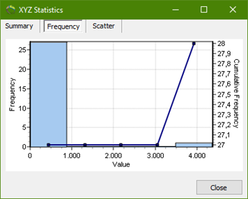
Figure 4. Distribution of chemical contaminant data. Clearly not Gaussian.

Figure 5. Select “Normal Score Transform” and press “Apply”.

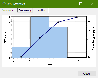
Figure 6. Data distribution after “Normal Score Transform” has been applied.

The statistics of the chemical contaminant, shown in Figure 4, is clearly not Gaussian. A large amount of the data values has very low concentrations of the chemical compound, while a significant amount has a very high concentration.

To use kriging correctly on these data, we have to perform a data transformation.

Close the Statistics window.

Select the “Normal Score Transformation”, as shown in Figure 5. Now press “Apply” and the values are transformed into normal score space.

Open the statistics window again to inspect the result, se Figure 6. The distribution of the transformed values now has a mean value of 0 and standard deviation (STD) of 1. A perfect Gaussian distribution.

You now complete the rest of the Wizard as you would normally do, noting that the estimation of the variogram is particularly easy now, as you now that your data have STD of 1, which corresponds to the Sill value of your variogram.

The program automatically handles the back transform of the interpolated values to normal space from Normal score space, so you do not have to worry about that.

Note: The variance grid constructed is an approximation, as the STD of the Kriging values are values in Normal Score Space.